Both error bars count
Spreadsheet trendlines ignore measurement uncertainty. curve.fit uses orthogonal distance regression (ODRPACK95, through the odrpack package) when students supply δx and δy, so every point is weighted by its uncertainty in both directions. With δy only it runs weighted least squares; with neither, ordinary least squares.
- Uncertainties come from a table column per point, or from a Rule: one constant or percentage for the whole dataset.
- Students choose how parameter uncertainties are reported. Absolute uses the supplied 1σ values as given. Nominal, the default, rescales by √χ²red, the same default as SciPy, lmfit and Origin.
- Parameters, the model uncertainty band and the reports show 1σ or 95% intervals. Residual plots carry error bars.
- Fit Statistics list the numbers of points and parameters, degrees of freedom, χ² and its p-value, AIC and BIC, and adjusted R² where it applies.
- Parameters can be fixed, or kept within lower and upper limits. A parameter that finishes on a limit is marked.
- Evaluate predicts y ± δy at any x, or solves for x from a measured y within the fitted range, propagating parameter uncertainty and an optional δx or δy. Lists of up to 100 values download as CSV.
| Uncertainties supplied | Fitting method | Checked against |
|---|---|---|
| None | Ordinary least squares in y | NIST reference datasets and a closed-form linear regression |
| δy only | Weighted least squares in y | An independent weighted linear regression, including parameter uncertainties |
| δx only | Orthogonal distance regression, exact-y limit | An independent regression of x on y, transformed back |
| δx and δy | Weighted orthogonal distance regression | The Pearson–York benchmark and an independent implementation of York’s equations |
Checked against published reference results
Before every release, an automated suite fits reference datasets with known answers and compares parameters, standard errors and residual sums of squares. The details, tolerances and references are published in the Help.
NIST Statistical Reference Datasets
21 datasets, 4 linear and 17 nonlinear, fitted from 55 certified and published starting points. Parameters, standard errors and residual sums of squares must match NIST’s certified values.
Pearson–York benchmark
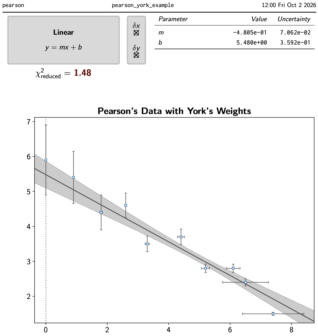
The classic test for fitting with errors in both variables: Pearson’s data with York’s weights, compared with the published results in Cantrell (2008). Load it in one click to show a class.
- Pearson, K. (1901). On lines and planes of closest fit to systems of points in space. Philosophical Magazine, 2, 559–572.
- York, D. (1966). Least-squares fitting of a straight line. Canadian Journal of Physics, 44, 1079–1086.
- Cantrell, C. A. (2008). Technical Note: Review of methods for linear least-squares fitting of data and application to atmospheric chemistry problems. Atmospheric Chemistry and Physics, 8, 5477–5487. doi:10.5194/acp-8-5477-2008
- NIST Statistical Reference Datasets, nonlinear and linear regression. nist.gov/itl/sed
- Zwolak, J. W., Boggs, P. T. & Watson, L. T. (2007). Algorithm 869: ODRPACK95: A weighted orthogonal distance regression code with bound constraints. ACM Transactions on Mathematical Software, 33(4), 27. doi:10.1145/1268776.1268782
A one-page report for every fit
Every fit exports a PDF with the model and equation, fitted parameters with 1σ or 95% uncertainties, reduced χ², the plot with error bars and uncertainty band, and the residuals.
- Single PDF for one report. Double PDF prints two copies side by side for lab partners.
- Titles and axis labels accept LaTeX math and symbols such as °, µ, ± and Greek letters, typeset with TeX. Custom equations are typeset as mathematics too.
- Browser Report opens the fit with full-precision tables, fit statistics and model samples, with CSV, JSON and Excel downloads for further analysis.
- An XLSX workbook holds the same full-precision tables and the plot, and the plot toolbar saves PNG or SVG images for slides.
- Each report is stamped with its session, fit ID and time, so an instructor can open the fit behind a submitted report.
Productive in minutes
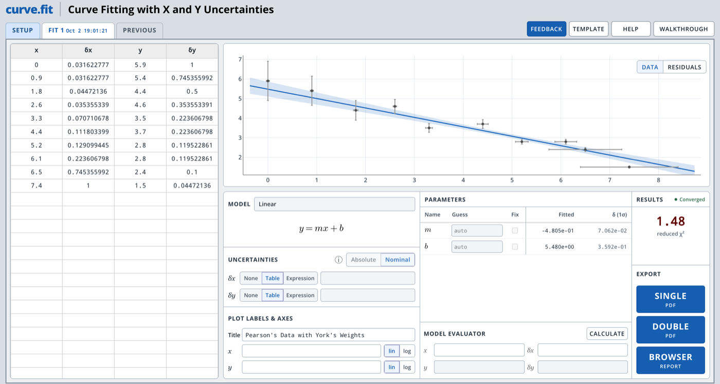
Paste the data
Copy x, δx, y and δy straight from a spreadsheet, or import a CSV file of up to 10,000 rows.
Choose a model
Pick one of 35 models or type an equation. Starting values are automatic.
Fit
Read the parameters, fit statistics and residuals. Each fit opens in its own tab.
Predict
Use Evaluate to get y ± δy at any x, or x from a measured y.
Export
Download the PDF for the lab report, an XLSX workbook, or the data as CSV.
- A guided walkthrough fits a sample dataset in about five minutes, in a separate practice tab.
- Custom equations use x and up to five parameters, A to E, with common functions and π. The equation is checked as students type, a matching built-in model is suggested when there is one, and saved fits and reports show it as typeset mathematics.
- Every fit is saved to a session link. Students can return later, compare fits of the same data by AIC in Previous, or fork a copy to try something new.
Models for physics, chemistry and biology labs
Every model has its own page with the equation, what each parameter means and tips for fitting it, and a link that opens the workspace with that model selected. The Custom Function page lists every function a custom equation can use.
Easy to adopt across sections
Instructor handout
Four pages for instructors and lab coordinators: comparisons with spreadsheets and Python, validation, the model library and custom equations, the Pearson–York example fitted with three uncertainty settings, and an annotated example report.
One method for every section
Every student uses the same fitting method and reporting conventions, whatever computer they have.
Share a dataset as a link
Fit an example once and share its session link. Reference examples such as Pearson–York and several NIST datasets load in one click.
Documented methods
The Help explains the fitting modes, uncertainty conventions, model bands and validation, with references students can cite. Short guides cover the background.
Reproducible in Python
A short SciPy template performs the same kind of ODR fit, for courses that want students to see the code.
Nothing to administer
No installs, licenses or student accounts. It runs in any modern browser on lab computers and laptops.
Free to use
There is no cost to students or departments, and no advertising.